Appendix H — Neural Network: Analytical Jacobian
Implementation status
| Model | DITL | PACE V3 | PACE V4 | Evaluation | Planned |
|---|---|---|---|---|---|
| AD Forward | — | — | — | x | — |
| AD Reverse | x | x | x | — | — |
The MAP retrievals are often computationally expensive due to their high dimensionality and iterative nature, with multiple forward model and Jacobian calculations. The data screening approach developed here further increases the demand for CPU computations because the retrieval must be repeated several times. Therefore, fast forward model and Jacobian matrix calculations are advantageous for efficient processing, which was a motivation for the use of NN forward models for AirHARP in Gao et al. (2021). In this work, we discuss the use of automatic differentiation to compute the Jacobian matrix analytically (Gao et al. 2021), as opposed to numerically through finite differencing, by exploiting the differentiable properties of the NN models. For details on the NN and its training strategies, please refer to Appendix G and discussions in Gao et al. (2021) and Gao et al. (2023).
The NN forward model developed in Gao et al. (2021) is a feed-forward neural network as defined in Table G.1, where \(\mathbf{h}_0=\mathbf{x}\) is the input layer that contains all 15 forward model parameters. Two sets of weight matrices \(\mathbf{W}_{p+1}\) and bias vectors \(\mathbf{b}_{p+1}\) have been determined from the NN training process for reflectance and DoLP, respectively (Gao et al. 2021, 2023).
Correspondingly, \(\mathbf{y}\) is the output layer for either reflectance or DoLP at the four AirHARP bands.
H.1 Mathematical formula of automatic differentiation
For application to multi-angle measurements, the NN needs to be called to simulate \(\mathbf{y}\) for each set of viewing and solar geometries for the state vector \(\mathbf{x}\) (Gao et al. 2021). Elements of the Jacobian matrix are defined as follows:
\[ \mathbf{K}_{mij} = \frac{\partial \mathbf{y}_{mi}} {\partial \mathbf{x}_{mj}} \tag{H.1}\]
Here, index \(m\) indicates the viewing and solar angles, index \(i\) indicates the wavelength, and index \(j\) indicates the state parameter. Table G.1 illustrates the structure of the NN.
Based on the the LeakyReLU activation function defined in Appendix G, its derivative with respect to each element in \(\Phi\) is defined as
\[ \mathbf{D}_{mi} = \frac{\Phi(\mathbf{Z})_{mi}} {\mathbf{Z}_{mi}} = \begin{cases} 1, & \mathbf{Z}_{mi}>0, \\ \alpha, & \mathbf{Z}_{mi}<0. \end{cases} \tag{H.2}\]
The forward operation of the NN is defined in Appendix G. During the forward pass, the intermediate values at each NN layer are stored and subsequently used to calculate the Jacobian through either forward-mode automatic differentiation (Table H.1) or reverse-mode automatic differentiation (backpropagation; Table H.2).
| Layers | AD: Forward mode |
|---|---|
| Input | \(\dot{\mathbf{h}}_{0,mij}=\delta_{ij}\) |
| Layer 1 | \(\dot{\mathbf{h}}_{1,mij}=\mathbf{D}_{1,mi}\mathbf{W}_{1,ij}^T\) |
| Layer \(p+1\) | \(\dot{\mathbf{h}}_{p+1,mij}=\mathbf{D}_{p+1,mi}\mathbf{W}_{p+1,il}^T\dot{\mathbf{h}}_{p,mlj}\) |
| Output | \(\mathbf{K}_{mij}=\dot{\mathbf{y}}_{mij}=\mathbf{W}_{k+1,il}^T\dot{\mathbf{h}}_{k,mlj}\) |
| Layers | AD: Reverse mode |
|---|---|
| Output | \(\bar{\mathbf{y}}_{mij}=\mathbf{W}_{k+1,ij}^T\) |
| Layer \(p+1\) | \(\bar{\mathbf{h}}_{p,mij}=\bar{\mathbf{h}}_{p+1,mil}\mathbf{D}_{p+1,ml}\mathbf{W}_{p+1,lj}^T\) |
| Layer 1 | \(\bar{\mathbf{h}}_{1,mij}=\bar{\mathbf{h}}_{2,mil}\mathbf{D}_{2,ml}\mathbf{W}_{2,lj}^T\) |
| Input | \(\mathbf{K}_{mij}=\bar{\mathbf{h}}_{0,mij}\) |
For brevity, summation over index \(l\) is implied following Einstein notation.
The finite difference (FD) method was used to compute the Jacobian matrix in FastMAPOL in Gao et al. (2021), where the NN forward model was called twice per input parameter under the central difference approximation of derivatives. To reduce the computational cost, the Jacobian matrix can be derived analytically from the NN forward model using AD based on the chain rule of differentiation (Baydin et al. 2018). Two recursive relations are obtained to compute the Jacobian matrix, as summarized in Table H.1 and Table H.2. The forward mode indicates the evaluation sequence from the first layer to the last layer, whereas the reverse mode indicates the evaluation sequence from the last layer to the first layer.
To represent the recursive relations, we define \(\dot{\mathbf{h}}_p\) (tangent) and \(\bar{\mathbf{h}}_p\) (adjoint) as follows:
\[ \dot{\mathbf{h}}_{p,mij} = \frac{\partial \mathbf{h}_{p,mi}} {\partial \mathbf{x}_{mj}}, \]
\[ \bar{\mathbf{h}}_{p,mij} = \frac{\partial \mathbf{y}_{mi}} {\partial \mathbf{h}_{p,mj}}. \]
Note that \(\mathbf{h}\) is defined in Table G.1 as the output from each hidden layer of the NN. The Jacobian matrix can be represented by AD with either the tangent or the adjoint form, corresponding to the final steps in Table H.1 and Table H.2, respectively:
\[ \mathbf{K}_{mij} = \dot{\mathbf{y}}_{mij} \tag{H.3}\]
\[ \mathbf{K}_{mij} = \bar{\mathbf{h}}_{0,mij} \tag{H.4}\]
where Equation H.3 and Equation H.4 are computed from forward- and reverse-mode AD, respectively. Forward and reverse AD produce identical results, but differ in computational efficiency because of the different sequence of matrix operations and the NN architecture.
For optimal efficiency, we implemented AD directly based on the formalism summarized in Table H.1 and Table H.2 using the PyTorch library (Paszke et al. 2019). The NN forward model is computed layer by layer, with the output from the previous layer serving as the input to the next layer, as summarized in Table G.1. Forward-mode AD follows the same sequence as the NN forward model, from the first layer to the last layer (Table H.1), whereas reverse-mode AD proceeds from the last layer backward to the first layer (Table H.2). Note that AD in both modes requires the values of matrix \(\mathbf{D}\) as defined in Equation H.2, which are determined by the output of the NN forward model at each layer.
For the NN used in this study, reverse-mode AD provides the highest computational efficiency, as investigated further in the next section.
The AD methods provide an efficient and accurate way to compute the Jacobian matrix, enabling substantial acceleration of retrieval algorithms such as FastMAPOL that involve a large number of state parameters and making them more suitable for practical applications.
H.2 Retrieval Efficiency Using Automatic Differentiation
The computational efficiency of FastMAPOL was evaluated using three approaches for calculating the Jacobian matrix: finite differences (FD) with central differencing, forward-mode automatic differentiation (AD), and reverse-mode AD.
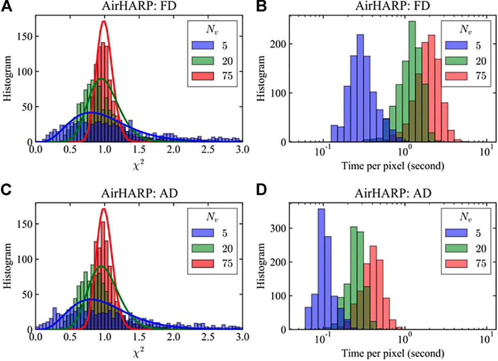
Figure H.1 compares the retrieved \(\chi^2\) distributions and computational times obtained using the different Jacobian methods in the example for HARP instrument Gao et al. (2021). The three approaches converge to similar \(\chi^2\) distributions, indicating that the use of AD does not appreciably affect the retrieval solution. The \(\chi^2\) distributions vary with the number of available viewing angles but can be well represented by the theoretical \(\chi^2\) distribution with the corresponding degrees of freedom. For reflectance and DoLP observations with the same number of viewing angles \(N_v\), the total number of measurements is \(N = 2N_v\).
The computational advantage of combining NN forward models with AD is substantial. Retrievals using the conventional radiative transfer model together with FD typically required approximately one hour to converge on a CPU (AMD EPYC processor). Replacing the radiative transfer calculations with NN forward models reduced the average retrieval time to approximately 3 s using the same FD approach .
Using AD further reduced the average CPU retrieval time to approximately 0.6 s with forward-mode AD and 0.3 s with reverse-mode AD, corresponding to an additional speedup of approximately 5–10 relative to the NN-based FD implementation. GPU processing further reduced the retrieval times to approximately 0.08 s and 0.05 s for forward- and reverse-mode AD, respectively.
| Forward Model | Jacobian Method | Hardware | Retrieval Time | Approximate Speedup |
|---|---|---|---|---|
| Radiative transfer | FD (central) | CPU | ~1 h | 1× |
| Neural network | FD (central) | CPU | ~3 s | ~1,200× |
| Neural network | AD (forward) | CPU | ~0.6 s | ~6,000× |
| Neural network | AD (reverse) | CPU | ~0.3 s | ~12,000× |
| Neural network | AD (forward) | GPU | ~0.08 s | ~45,000× |
| Neural network | AD (reverse) | GPU | ~0.05 s | ~72,000× |
Among the tested approaches, reverse-mode AD provides the highest computational efficiency. FastMAPOL therefore uses reverse-mode AD as the default method for calculating the Jacobian matrix during retrieval optimization. Further speed up is discussed by the use of cascading NN for first guess and full retrievals Appendix G.