Appendix G — Neural Network: Model and Training
Implementation status
| Model | DITL | PACE V3 | PACE V4 | Evaluation | Planned |
|---|---|---|---|---|---|
| - | x | x | x | — | — |
FastMAPOL uses deep feed-forward neural networks (NNs) as computationally efficient emulators of the vector radiative transfer (RT) forward model. Separate NNs are trained for reflectance (\(\rho\)) and degree of linear polarization (DoLP, \(P\)), allowing their different angular characteristics and accuracy requirements to be treated independently. The general NN methodology follows Gao et al. (2021), with subsequent improvements for PACE polarimeter retrievals described in Gao et al. (2023).
G.1 Training Data
The NN training data are generated from the high-accuracy vector RT simulations described in the previous section. The training parameter space covers the aerosol, ocean surface, atmospheric, and observation-geometry parameters required by the FastMAPOL forward model. Compared with the earlier AirHARP implementation (Gao et al. 2021), the PACE implementation extends the parameter space to include aerosol layer height (ALH) and surface pressure and covers a larger range of viewing geometries [Gao et al. (2023); Gao:2026aa]. The latter is enabled by the improved pseudo-spherical shell (IPSS) correction (Zhai and Hu 2022) and the use of viewing geometry defined at the Earth’s surface.
A total of 10,000-20,000 independent RT cases are generated by randomly sampling the model input parameters over their prescribed ranges, depending on the accuracy requirement and complexities of the RT system. Aerosol optical depth (AOD) is often niformly sampled between 0.01 and 0.5 and is used, together with the sampled aerosol size and composition parameters, to determine the aerosol volume densities following the strategy described in Gao et al. (2021). Note that the NN can be still used for AOD larger than 0.5, but the sampling is not optimal as the range less than 0.5, and have showing a negative bias in the retrievals (Gao et al. 2026). Further expansions are planned for future versions.
A single RT simulation provides radiances over a large number of viewing geometries. This allows multiple viewing directions to be sampled from each RT case and substantially increases the effective size of the NN training dataset without requiring additional full RT calculations. This approach is analogous to data augmentation in machine learning.
For example for the training of NN for HARP2, sets of 100, 400, and 1000 viewing geometries are sampled from each of the 10,000 RT simulations, resulting in approximately 1 million, 4 million, and 10 million training samples, respectively. The impact of this data augmentation on NN accuracy was systematically evaluated in Gao et al. (2023).
G.2 Neural Network Architecture
A feed-forward NN with \(k\) hidden layers can be expressed recursively as summarized in Table G.1.
| Layer | NN forward model |
|---|---|
| Input | \(\mathbf{h}_0=\mathbf{x}\) |
| Layer 1 | \(\mathbf{h}_1=\Phi(\mathbf{W}_1^T\mathbf{h}_0+\mathbf{b}_1)\) |
| Layer \(p+1\) | \(\mathbf{h}_{p+1}=\Phi(\mathbf{W}_{p+1}^T\mathbf{h}_p+\mathbf{b}_{p+1})\) |
| Output | \(\mathbf{y}=\mathbf{W}_{k+1}^T\mathbf{h}_k+\mathbf{b}_{k+1}\) |
Here, \(\mathbf{x}\) is the forward-model input vector, \(\mathbf{y}\) contains the NN-predicted reflectance or DoLP, \(\mathbf{W}_p\) and \(\mathbf{b}_p\) are the trainable weight matrices and bias vectors, and \(\mathbf{h}_p\) is the output of hidden layer \(p\).
The nonlinear activation function \(\Phi\) is the LeakyReLU function, applied element-wise as
\[ \Phi(\mathbf{Z})_{mi} = \max(0,\mathbf{Z}_{mi}) + \alpha\min(0,\mathbf{Z}_{mi}), \tag{G.1}\]
where \(\alpha=0.01\), and \(m\) and \(i\) denote the matrix indices of \(\mathbf{Z}\). LeakyReLU was selected because it provided slightly better accuracy than the standard ReLU activation in the NN training experiments (Gao et al. 2021).
For the PACE implementation described in Gao et al. (2023), the primary reflectance and DoLP NNs contain 17 inputs and 4 outputs. Multiple architectures were evaluated, ranging from two hidden layers with 64 or 128 nodes per layer to three hidden layers with 128, 256, or 512 nodes per layer. For convenience, an architecture with three hidden layers containing 256 nodes each is denoted as \(256^3\).
G.3 Training Procedure
The NN inputs and outputs are normalized before training to reduce differences in scale among the forward-model parameters and output quantities. The NN parameters are optimized using mini-batch training. A batch size of 1024 is used, and the Adam optimization algorithm (Kingma and Ba 2015) is applied to update the NN weights and biases. The NN models are implemented and trained using PyTorch (Paszke et al. 2019).
The simulated dataset is randomly divided into 70% for training and 30% for validation. The training subset is used to optimize the NN parameters, while the independent validation subset is used to monitor generalization and identify overfitting. Increasing both the number of training samples and the NN size was found to reduce the training and validation errors, with the larger augmented datasets substantially reducing the difference between the two.
G.4 Measurement-Uncertainty-Aware Training
A key improvement in the PACE FastMAPOL NN training is the use of a measurement-uncertainty-aware cost function (Gao et al. 2023).
Conventional NN training minimizes a mean squared error (MSE) between the RT simulations and NN predictions. This approach can be problematic for ocean reflectance because the sunglint signal can become strongly peaked at low wind speeds. The large magnitude of reflectance near the specular direction can dominate the MSE and reduce the relative importance of other viewing geometries.
Earlier implementations addressed this problem by excluding observations near the specular reflection direction from the training data (Gao et al. 2021). However, removing sunglint observations also eliminates information useful for retrieving ocean surface wind speed and aerosol properties (Gao et al. 2021).
FastMAPOL instead retains these observations and normalizes the NN residuals by the assumed measurement uncertainties. The training cost functions for reflectance and DoLP are defined as
\[ \chi^2_{\mathrm{NN},\rho} = \frac{1}{N} \sum_i \frac{ \left[ \rho_t(i)-\rho_t^{\mathrm{NN}}(\mathbf{x};i) \right]^2 }{ \sigma_\rho^2(i) }, \]
and
\[ \chi^2_{\mathrm{NN},P} = \frac{1}{N} \sum_i \frac{ \left[ P_t(i)-P_t^{\mathrm{NN}}(\mathbf{x};i) \right]^2 }{ \sigma_P^2(i) }, \]
where \(\rho_t\) and \(P_t\) are the RT-generated training values, \(\rho_t^{\mathrm{NN}}\) and \(P_t^{\mathrm{NN}}\) are the corresponding NN predictions, and \(N\) is the number of samples in a training batch.
The uncertainty model used for NN training follows that used in the retrieval:
\[ \sigma_\rho = 0.03\rho_t, \qquad \sigma_P = 0.005. \]
For reflectance, this formulation approximately represents a relative or percentage fitting error and prevents the large absolute magnitude of sunglint reflectance from dominating the optimization. It therefore allows both sunglint and non-sunglint geometries to be represented within the same training framework.
For DoLP, \(\sigma_P\) is constant, so the uncertainty-normalized cost function is mathematically equivalent to a scaled MSE. Because DoLP remains bounded and does not exhibit the same large-magnitude sunglint behavior as reflectance, its training is less affected by this issue.
An additional advantage of this formulation is that the NN training accuracy can be interpreted directly relative to the measurement uncertainty. For example,
\[ \chi^2_{\mathrm{NN}}=0.01 \]
corresponds to a typical NN residual of approximately
\[ \sqrt{0.01}=0.1 \]
times the assumed measurement uncertainty.
G.5 Training Performance and NN Selection
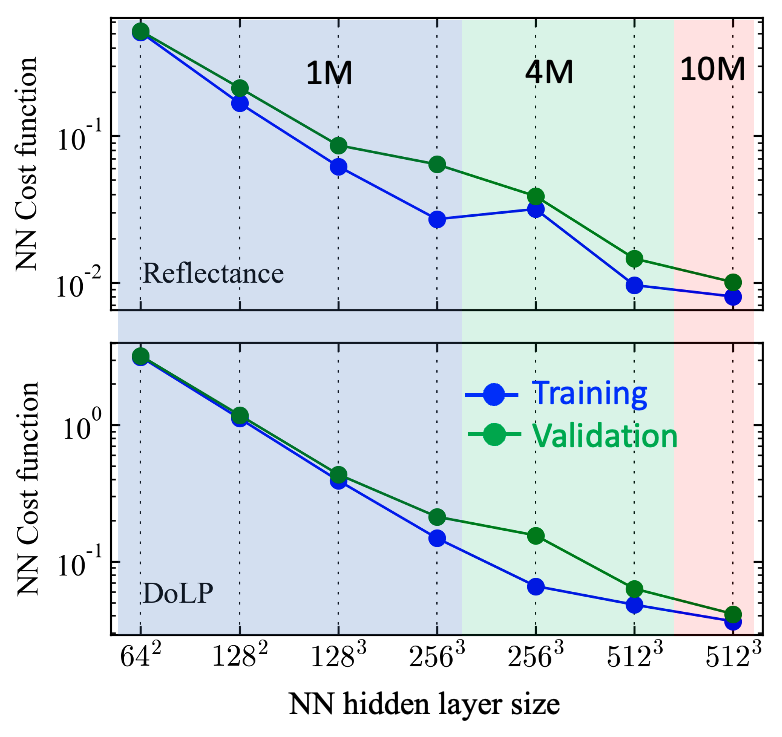
The effects of NN architecture and training-data size were systematically evaluated using datasets containing 1 million, 4 million, and 10 million samples. Increasing the NN size generally decreases both the training and validation cost functions. However, for smaller training datasets, sufficiently large networks can begin to overfit, as indicated by a validation cost larger than the training cost.
Increasing the augmented training dataset from 1 million to 4 million and ultimately 10 million samples reduces this difference and allows larger NN architectures to be effectively trained. With 10 million samples, the reflectance NN converges to a cost function of approximately 0.01. This corresponds to a typical NN residual of approximately 0.1 times the assumed 3% reflectance measurement uncertainty, or about 0.3%.
DoLP requires a larger NN to reach a comparable normalized training accuracy because the assumed DoLP measurement uncertainty, 0.005, imposes a more stringent absolute accuracy requirement. With 10 million samples and a \(512^3\) architecture, the DoLP cost function is approximately 0.04, corresponding to an NN error of approximately
\[ \sqrt{0.04}\times0.005 = 0.001. \]
A similar level of normalized accuracy for reflectance can be achieved with the smaller \(256^3\) architecture.
G.6 Cascaded Neural Network Forward Model
FastMAPOL uses a two-level cascaded NN scheme to balance computational efficiency and forward-model accuracy.
Also with the example of NN training with HARP2 data in Gao et al. (2023), in the first retrieval stage, relatively compact NNs are used to rapidly approach the solution:
- Reflectance: \(64^2\)
- DoLP: \(128^2\)
The resulting state vector is then used as the initial condition for a second retrieval stage employing higher-accuracy NNs:
- Reflectance: \(256^3\)
- DoLP: \(512^3\)
Each retrieval stage itself involves multiple nonlinear optimization iterations. The smaller first-stage NNs therefore reduce the computational cost of iterations performed while the solution is still relatively far from the optimum, whereas the larger second-stage NNs provide the accuracy required near the final solution.
Tests comparing single-level and two-level retrievals show similar retrieval uncertainties when the same high-accuracy NN is used in the final stage. The cascade therefore improves computational efficiency without appreciably affecting retrieval accuracy.
The NN representation also enables the Jacobian matrix required by the nonlinear optimization to be calculated analytically using automatic differentiation and the chain rule (Gao et al. 2021) with more discussion in Appendix H, avoiding the substantially larger computational cost of finite-difference Jacobians.
G.7 Independent Evaluation of NN Accuracy
In addition to the training and validation datasets, NN accuracy was evaluated using 1000 independent RT simulations with realistic HARP viewing geometries that were not used during NN training. The NN predictions were compared directly with the corresponding high-accuracy RT simulations using metrics including the mean absolute error (MAE) and root mean square error (RMSE):
\[ \mathrm{MAE} = \frac{1}{N} \sum_{i=1}^{N} \left|R_i-T_i\right|, \]
\[ \mathrm{RMSE} = \sqrt{ \frac{1}{N} \sum_{i=1}^{N} \left(R_i-T_i\right)^2 }, \]
where \(T_i\) represents the RT simulation and \(R_i\) represents the corresponding NN prediction.
MAE is less sensitive to a small number of large residuals and was therefore found to provide a robust characterization of the typical NN error. Based on this independent evaluation, the reflectance uncertainty for the \(512^3\) NN is approximately 0.5%, while the corresponding DoLP uncertainty is approximately 0.002. These estimates are slightly larger than, but generally consistent with, those inferred directly from the uncertainty-normalized training cost functions.
The RT calculations used to generate the training data are configured with numerical accuracy substantially better than both the measurement uncertainty and NN approximation error for HARP2 [Gao et al. (2021); Gao:2023aa] and SPEXone [Gao:2026aa]. Consequently, the NN forward models provide an efficient approximation of the full vector RT calculations while maintaining the accuracy required for FastMAPOL retrievals. For application to measured data, the complete uncertainty budget should account for measurement uncertainty, NN approximation uncertainty, and RT-model numerical uncertainty.