Appendix I — Uncertainty Quantification: Theory
Implementation status
| Model | DITL | PACE V3 | PACE V4 | Evaluation | Planned |
|---|---|---|---|---|---|
| — | x | — | — | — | — |
The uncertainty framework propagates uncertainties associated with the measurements and forward model through the retrieval based on the sensitivity of the forward model to the retrieved state parameters. Corresponding uncertainty products were generated for the global Day-In-The-Life (DITL) test dataset and are available through OB.DAAC (Gao et al. 2023). However, because of the additional computational cost associated with uncertainty propagation, these uncertainty variables are not included in the current FastMAPOL V3 and V4 operational products and are planned for a future release.
This chapter reviews the methodology for pixel-level uncertainty quantification through error propagation and describes approaches for evaluating and validating the resulting uncertainty estimates.
The approach follows the error-propagation framework of Rodgers (2000) and uses the Jacobian matrix calculated from the neural-network (NN) forward model through automatic differentiation (AD). This enables uncertainties to be calculated efficiently for both directly retrieved state parameters and derived geophysical products.
I.1 Input Uncertainty Model
The FastMAPOL retrieval minimizes the difference between the measurements and forward-model calculations using the normalized cost function as discussed in Appendix D.
Note that the error covariance matrix \(\mathbf{S}_{\epsilon}\) describes the uncertainties associated with the measurements and forward model. The diagonal uncertainty \(\sigma_{\epsilon}\) for each observation includes contributions from the instrument \(\sigma_{\mathrm{ins}}\), NN approximation \(\sigma_{\mathrm{NN}}\), and numerical accuracy of the radiative transfer (RT) simulation \(\sigma_{\mathrm{RT}}\). These contributions are assumed to be mutually independent.
The current implementation assumes that the measurement errors are uncorrelated, such that \(\mathbf{S}_{\epsilon}\) is diagonal. This assumption simplifies the uncertainty propagation and retrieval optimization. Correlated spectral and angular uncertainties can be represented through the off-diagonal elements of \(\mathbf{S}_{\epsilon}\) when such information is quantifized (Appendix J)
Additional forward-model errors resulting from incomplete physical representation of the observed scene are not explicitly included. FastMAPOL uses adaptive multi-angle screening to identify and remove observations that cannot be adequately represented by the forward model, thereby reducing the influence of these modeling errors on the retrieval.
I.2 Pixel-Level Retrieval Uncertainty
FastMAPOL estimates the theoretical uncertainty for each individual retrieval by propagating the input uncertainties into the retrieved state space.
Under the local linearity and Gaussian-error assumptions, the retrieval covariance matrix is approximated by
\[ \mathbf{S}^{-1} = \mathbf{K}^T \mathbf{S}_{\epsilon}^{-1} \mathbf{K} + \mathbf{S}_{a}^{-1}, \tag{I.1}\]
where \(\mathbf{S}\) is the retrieval covariance matrix, \(\mathbf{S}_{\epsilon}\) is the input error covariance matrix, \(\mathbf{K}\) is the Jacobian matrix, and \(\mathbf{S}_{a}\) represents the effective prior covariance matrix.
The Jacobian matrix describes the sensitivity of each modeled observation to each retrieved state parameter:
\[ K_{ij}(\mathbf{x}) = \frac{\partial F_i(\mathbf{x})}{\partial x_j}, \tag{I.2}\]
where index \(i\) represents a measurement and index \(j\) represents a retrieved parameter.
The \(1\sigma\) uncertainty of a directly retrieved parameter \(x_j\) is obtained from the corresponding diagonal element of the retrieval covariance matrix:
\[ \sigma_{x_j} = \sqrt{S_{jj}}. \tag{I.3}\]
The off-diagonal elements of \(\mathbf{S}\) describe the error covariance among retrieved parameters and therefore provide information on parameter coupling within the inversion.
I.3 Treatment of Retrieval Bounds
FastMAPOL does not use explicit a priori state information as an additional term in the retrieval cost function. Instead, each state parameter is constrained to a physically meaningful range during the nonlinear least-squares optimization.
These retrieval bounds act as implicit prior constraints. For uncertainty propagation, \(\mathbf{S}_{a}\) is approximated as a diagonal matrix based on the permitted range of each state parameter. This prevents the propagated uncertainty from becoming substantially larger than the physically plausible parameter range.
This treatment is an approximation to the Bayesian formalism of Rodgers (2000). For well-constrained retrievals, the measurement information dominates Equation I.1 and the assumed prior covariance generally has little numerical effect.
I.4 Uncertainty of Derived Geophysical Products
Many FastMAPOL products are derived from the retrieved state vector rather than retrieved directly. Examples include aerosol optical depth (AOD), single-scattering albedo (SSA), and quantities derived through atmospheric correction.
For a derived quantity
\[ a=a(\mathbf{x}), \]
its uncertainty is propagated from the full state covariance matrix as
\[ \sigma_a = \sqrt{ \sum_i \sum_j S_{ij} \frac{\partial a}{\partial x_i} \frac{\partial a}{\partial x_j} }. \tag{I.4}\]
Equivalently, defining the gradient
\[ \mathbf{g}_a = \frac{\partial a}{\partial\mathbf{x}}, \]
the propagated variance can be written compactly as
\[ \sigma_a^2 = \mathbf{g}_a^T \mathbf{S} \mathbf{g}_a. \tag{I.5}\]
This formulation retains the covariance among retrieved state parameters. Neglecting the off-diagonal elements of \(\mathbf{S}\) can therefore produce different uncertainty estimates when the derived quantity depends on multiple correlated retrieval parameters.
FastMAPOL uses automatic differentiation to calculate the derivatives required in Equation I.2 and Equation I.4. This approach is applied to derived aerosol properties such as AOD and SSA as well as quantities associated with atmospheric correction.
I.5 Automatic Differentiation for Uncertainty Propagation
Calculation of the Jacobian matrix can be computationally expensive when conventional finite differences (FD) are used. For a state vector containing many parameters, the forward model must be evaluated repeatedly after perturbing each parameter.
Because the FastMAPOL forward model is represented by differentiable neural networks, the required derivatives can instead be calculated analytically through automatic differentiation. AD applies the chain rule directly through the NN operations and avoids the repeated perturbation calculations required by FD as discussed in Appendix H.
The same framework can be used to calculate both
- the forward-model Jacobian \(\mathbf{K}\) required for retrieval optimization and Equation I.1, and
- the derivatives of derived products with respect to the state vector required by Equation I.4.
Reverse-mode AD provides particularly high computational efficiency for the FastMAPOL retrieval and is therefore used as the default approach for Jacobian and uncertainty calculations.
This allows pixel-level uncertainties to be produced as an integral part of the retrieval rather than through a separate computationally expensive uncertainty analysis.
I.6 Interpretation of Theoretical Uncertainty
The propagated uncertainties represent the expected \(1\sigma\) dispersion of the retrieved quantities under the assumptions of the uncertainty model and the local linearization of the forward model.
These theoretical uncertainties do not necessarily capture every source of retrieval error. Differences between theoretical uncertainty and actual retrieval performance can arise from several factors, including:
- incomplete or inaccurate representation of the physical scene by the forward model,
- uncertainties or correlations not represented in \(\mathbf{S}_{\epsilon}\),
- nonlinearities in the forward model,
- insufficient measurement information for separating correlated state parameters,
- convergence to a local rather than global minimum,
- retrieval parameters approaching imposed physical boundaries, and
- numerical convergence criteria used by the nonlinear optimization.
Consequently, theoretical uncertainty estimates should be evaluated against retrieval errors obtained from synthetic experiments or independent validation measurements whenever possible.
I.7 Evaluation of Retrieval Uncertainty
For synthetic retrieval experiments, retrieval errors can be calculated directly because the true state is known. For validation against independent measurements, the corresponding reference observations can be used as an estimate of truth, with their own uncertainties considered when interpreting the comparison.
Two useful metrics for characterizing retrieval errors are the root mean square error (RMSE) and mean absolute error (MAE):
\[ \mathrm{RMSE} = \sqrt{ \frac{1}{M} \sum_{i=1}^{M} (R_i-T_i)^2 }, \tag{I.6}\]
and
\[ \mathrm{MAE} = \frac{1}{M} \sum_{i=1}^{M} |R_i-T_i|, \tag{I.7}\]
where \(R_i\) is the retrieved value, \(T_i\) is the corresponding reference value, and \(M\) is the number of retrieval cases.
For a zero-mean Gaussian error distribution,
\[ \mathrm{RMSE} = \sqrt{\frac{\pi}{2}} \,\mathrm{MAE}. \tag{I.8}\]
MAE is generally less sensitive to outliers than RMSE. Comparing the two metrics therefore provides information about whether the observed retrieval-error distribution is consistent with a Gaussian distribution.
I.8 Monte Carlo Error Propagation
Direct comparison between pixel-level theoretical uncertainties and observed retrieval errors is not straightforward. The theoretical uncertainty represents the expected standard deviation of a probability distribution for an individual retrieval, whereas the observed error is a single realization of that distribution.
One component in FastMAPOL is to use a sampling-based approach, referred to as Monte Carlo Error Propagation (MCEP), to place theoretical and observed retrieval errors into a common statistical framework as discussed in Gao et al. (2022).
For each retrieval with theoretical uncertainty \(\sigma_i\), a random theoretical error is sampled as
\[ e_i^{\mathrm{theory}} \sim \mathcal{N}(0,\sigma_i^2). \tag{I.9}\]
The resulting ensemble of sampled errors represents the error distribution expected from the pixel-level theoretical uncertainties.
The MCEP procedure consists of the following steps:
Perform the retrieval and calculate pixel-level uncertainty.
For each retrieval, calculate the theoretical \(1\sigma\) uncertainty using Equation I.1 or Equation I.4.Sample theoretical retrieval errors.
For each case, generate a random error from a zero-mean Gaussian distribution with standard deviation equal to its theoretical uncertainty.Calculate observed retrieval errors.
Determine the actual retrieval error from the difference between the retrieved and reference values:\[ e_i^{\mathrm{obs}}=R_i-T_i. \]
Compare the error distributions.
Compare the sampled theoretical and observed error distributions using statistics such as MAE, RMSE, percentiles, or their complete probability distributions.Evaluate statistical variability.
Repeat the random sampling to estimate the uncertainty of the ensemble metrics themselves. This is particularly important when only a limited number of validation cases are available.
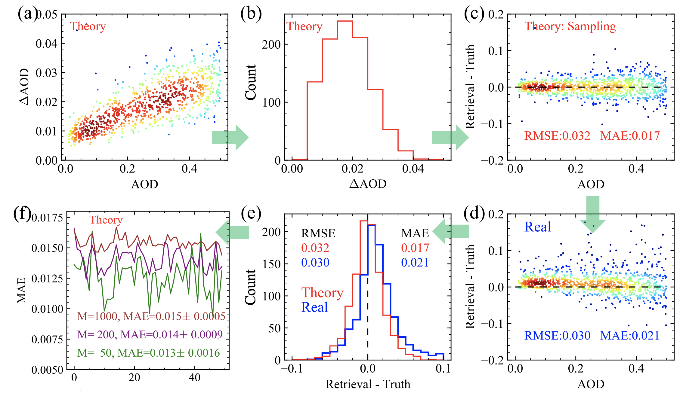
MCEP therefore converts a collection of heterogeneous pixel-level uncertainties into an ensemble error distribution that can be compared directly with the observed retrieval-error distribution.
Importantly, the method does not require the distribution of the retrieved geophysical quantity itself, such as AOD, to be Gaussian. Each individual theoretical uncertainty is used to generate its own conditional error distribution, and the resulting ensemble may have a substantially non-Gaussian shape.
I.9 Uncertainty for Logarithmically Distributed Quantities
Some retrieved quantities, particularly chlorophyll-a concentration (Chla), span several orders of magnitude and are more appropriately evaluated in logarithmic space.
Following Seegers et al. (2018), a logarithmic MAE metric can be defined as
\[ \mathrm{MAE(log)} = 10^Y, \]
where
\[ Y = \frac{1}{M} \sum_{i=1}^{M} \left| \log_{10}(R_i) - \log_{10}(T_i) \right|. \tag{I.10}\]
A value of \(\mathrm{MAE(log)}=1.2\), for example, represents a typical multiplicative difference of approximately 20%.
To compare the theoretical Chla uncertainty with errors expressed in logarithmic space, the propagated uncertainty can be transformed as
\[ \sigma_{\log_{10}(\mathrm{Chla})} = \frac{ \sigma_{\mathrm{Chla}} }{ \mathrm{Chla}\ln(10) }. \tag{I.11}\]
This transformation allows the pixel-level theoretical uncertainty and validation statistics to be evaluated consistently for quantities spanning a large dynamic range.
I.10 Summary
The FastMAPOL uncertainty framework provides pixel-level uncertainty estimates that are physically connected to the measurement information and the sensitivity of the forward model. The principal components of the framework are:
- an input uncertainty model incorporating measurement, NN, and RT numerical uncertainties;
- Jacobian-based propagation of input uncertainties into the retrieved state vector;
- full covariance information describing uncertainty and coupling among retrieved parameters;
- propagation of the state covariance to derived products such as AOD and SSA;
- efficient calculation of the required derivatives using automatic differentiation; and
- statistical evaluation of theoretical uncertainties against synthetic or validation data using MCEP.
Together, these components provide both an uncertainty estimate for future FastMAPOL retrieval and a framework for evaluating whether those theoretical uncertainties are representative of observed retrieval performance.